Design tools: soliton numbers and dispersive-wave phase matching#
Estimate the dispersion, nonlinear length and likely emission wavelengths before choosing a propagation window. The design tools turn a mode, fill and pulse into useful starting parameters; their assumptions determine how to interpret those estimates. A phase-matching root locates a possible emission frequency, not its conversion efficiency.
The soliton lesson connects soliton order to pulse evolution, and the RDW lesson shows emission in a changing gas fill. This chapter gives the corresponding calculators and equations. Quantities use SI, with pressure accepted in bar at the user interface. The final section compares the estimates with propagation.
The soliton numbers#
For a pulse of energy \(E\) and full width at half maximum \(\tau_{\rm fwhm}\) (of the power) at angular frequency \(\omega_0\), in a mode with group-velocity dispersion \(\beta_2\) and effective area \(A_{\rm eff}\), filled with a gas of nonlinear index \(n_2\):
The natural width \(\tau_0\) and the peak power \(P_0\) depend on the pulse shape:
shape |
\(\tau_0\) |
\(P_0\) |
|---|---|---|
|
\(\tau_{\rm fwhm}/(2\ln(1+\sqrt2))\) |
\(E/(2\tau_0)\) |
|
\(\tau_{\rm fwhm}/(2\sqrt{\ln 2})\) |
\(E/(\sqrt\pi\,\tau_0)\) |
One shape is used through the whole chain (pulse_width(),
pulse_peak_power(),
dispersion_length(),
soliton_order(), fission_length()), so a
Gaussian’s soliton order is computed from the Gaussian width and the Gaussian peak power
throughout.
soliton_params() collects all of it for any mode and any fill,
and capillary_params() builds the capillary mode for you, exactly
as prop_capillary() would for the same arguments:
>>> from solprop.tools import capillary_params
>>> p = capillary_params(125e-6, "He", 0.4, energy=300e-6, fwhm=10e-15,
...                      wavelength=800e-9, cladding=1.45)
>>> print(p)
MODE:
  MarcatiliMode(HE11, a=125 um, He, model=full, loss=True)
WAVEGUIDE:
  Aeff = 2.34e-08 m^2, Lloss = 7.05e+00 m (1/e power)
FILL:
  0.4 bar He at 293.15 K, Pcr = 6.52e+11 W,
  gamma = 4.88e-11 /(W m), n2 = 1.45e-21 cm^2/W
PULSE:
  3.000e-04 J, 1.000e-14 s @ 800.0 nm (shape: sech)
DISPERSION:
  -8.103e-30 s^2/m @ 800.0 nm, ZDW = 376.7 nm
POWER:
  2.64e+10 W (0.0406 of Pcr)
INTENSITY:
  1.13e+14 W/cm^2 mode-averaged, 2.00e+14 W/cm^2 on axis
SOLITON:
  Ld = 3.97e+00 m, Lnl = 7.74e-01 m, Lfiss = 1.75e+00 m, N = 2.26
CONSTITUENTS (unchirped NLSE):
  2 discrete solitons, area/pi = 2.26
  largest P = 6.422e+10 W, T = 1.607e-15 s, kNL = 1.568e+00 1/m
The result is a frozen
SolitonParams whose fields are SI and spelled out
(soliton_order, fission_length, critical_power, …).
Three of its entries need a word of explanation.
Two intensities. intensity is \(P_0/A_{\rm eff}\), the mode-averaged value.
peak_intensity is the intensity on the axis, which is relevant to local ionisation and to
the peak_intensity statistic of a resolved capillary run; for the fundamental of a capillary it
is 1.77 times larger. In a mode-averaged model the nonlinear response samples an
effective-area field instead; do not equate that with a resolved on-axis rate. It is built from the same normalised mode profile the run uses,
and a test compares it with the first plane of a run.
The zero-dispersion wavelength is searched, not bracketed once. A gas resonance in
the vacuum ultraviolet flips the sign of \(\beta_2\) twice (krypton near 120 nm), so a
single bracket over 100 nm to 3 µm sees the same sign at both ends and finds nothing.
The dispersion is sampled, each sign change refined, the changes through a pole
discarded (there \(\beta_1\) diverges; at a zero it is extremal), and the zero nearest the
pump reported. When there is none the field is nan and the block says so.
Note
The modes’ own zdw(), and the zdw statistic that uses
it, do not search this way: they test only the signs of \(\beta_2\) at the ends of the
window before a bracketed root search, so an even number of interior zeros — two
zero-dispersion wavelengths, or a resonance’s pair of sign changes as in krypton or
xenon — reads as no zero, and the search raises. Use the design tools’ search for such a
case.
The critical power is self_focusing_power(),
\(P_{\rm cr}=1.86226\,\lambda^2/(4\pi n_0n_2)\) (Fibich and Gaeta, Opt. Lett. 25, 335
(2000)). It is solprop.spatial.critical_power() evaluated at index=n0: both
measure the physical axial power in the medium, and the package has one Townes
constant.
gas_ratio() compares two gases at one wavelength, pressure and
temperature — the ratio of their bulk dispersions and of their Kerr responses, by name —
for the “what pressure of argon matches this helium” question.
The solitons actually excited#
The conventional \(N=\sqrt{L_D/L_{NL}}\) is a continuous measure of nonlinearity.
It is not generally the number of discrete solitons. In particular, a Gaussian
with conventional \(N=1\) is not a fundamental sech soliton.
soliton_content() calculates the count and the largest
constituent for an unchirped sech or Gaussian input in anomalous dispersion.
SolitonParams.soliton_content exposes the same result; in normal dispersion it
is None, while the conventional design numbers remain available.
With \(x=t/\tau_0\) and the focusing NLSE normalisation \(i u_\zeta+\tfrac12u_{xx}+|u|^2u=0\), the input fields are \(q(x)=N\,\mathrm{sech}(x)\) and \(q(x)=N e^{-x^2/2}\). For these real single-lobe profiles, the area theorem gives
Here \(M\) counts strictly positive discrete eigenvalues. At \(S=j+1/2\) the new zero eigenvalue is not a square-integrable soliton and is excluded. The first Gaussian soliton therefore requires \(N>\sqrt{\pi/8}\). This is the single-lobe result of Klaus and Shaw, not an area rule for arbitrary chirped or multi-peaked fields.
For sech input the largest eigenvalue is \(i\eta\), \(\eta=N-1/2\) when positive. For Gaussian input we solve the Zakharov-Shabat scattering problem; there is no substitution of an energy-equivalent sech pulse or a WKB approximation. Kim, Lee and Lyng distinguish the numerical Gaussian eigenvalues from the semiclassical WKB estimates. Writing the real Jost vector as \(r(\cos\theta,\sin\theta)\) gives
The largest eigenvalue satisfies \(\theta(0)=-\pi/4\). Integrating this angle avoids exponential amplitude growth. The omitted Gaussian field area is at most \(10^{-13}\); DOP853 uses relative tolerance \(10^{-11}\) and absolute tolerance \(10^{-13}\). Brent refinement has the same relative tolerance and \(10^{-13}\) absolute tolerance on \(\eta\). Tests compare against independent left/right amplitude matching and longer intervals. Close to the first threshold relative eigenvalue accuracy degrades; an unresolved positive eigenvalue raises rather than returning a fictitious zero-power soliton.
The constituent is a fundamental sech soliton with
For example, a Gaussian with conventional \(N=1\) has one constituent with
\(\eta\simeq0.4207333\) and \(P_{\max}\simeq0.7080661P_0\); a sech with \(N=3\)
has three constituents and \(P_{\max}=25P_0/9\). The rest of a Gaussian’s energy
is shared among the other constituents, when present, and dispersive radiation.
These are lossless cubic-NLSE scattering quantities, not a simulation of
perturbed fission. fission_length remains the conventional estimate \(L_D/N\).
Where the dispersive wave comes out#
A fundamental soliton of peak power \(P_0\) in a mode with propagation constant \(\beta_{\rm s}\) is, in the frame moving at its group velocity,
It does not disperse, so every frequency component of it advances with the same phase: the component at \(\omega\) has the wavenumber
A linear wave at \(\omega\) in a mode with propagation constant \(\beta_{\rm dw}\) is driven resonantly by the soliton’s spectral tail where the two wavenumbers agree (Akhmediev and Karlsson, Phys. Rev. A 51, 2602 (1995)), that is where
phase_mismatch() is this function.
lambda_rdw() finds its longest root inside a wavelength window —
by default 100 nm to 0.9 of the pump wavelength, where that is the short-wavelength wave
nearest the pump — and lambda_rdw_all() every root.
With pulse data, the default nonlinear_phase="largest" uses the phase of the
largest constituent calculated above: supply input peak_power, gamma, fwhm
and shape. The input duration is required; it is not inferred from peak power.
For sech input this gives \(k_{\rm NL}=\gamma P_0(2N-1)^2/(2N^2)\).
For Gaussian input the eigenvalue determines the constituent’s power.
To use a specified fundamental-soliton power instead, pass
nonlinear_phase="supplied_power", peak_power and gamma, omitting fwhm; the
nonlinear wavenumber is then \(\gamma P_0/2\). With no pulse numbers the calculation
remains linear; nonlinear_phase="linear"
selects this explicitly and requires omitting the pulse numbers. Inconsistent
arguments, normal dispersion or an input below the soliton threshold are refused
for the constituent calculation. In intermodal matching, its dispersion and Kerr
coefficient belong to the soliton mode.
The following plot uses the supplied-power option to compare that fundamental-soliton estimate with the linear condition.
import warnings

import matplotlib.pyplot as plt
import numpy as np

from solprop.exceptions import MaterialRangeWarning
from solprop.modes import MarcatiliMode
from solprop.physdata import n2
from solprop.tools import lambda_rdw, nonlinear_coefficient, phase_mismatch

mode = MarcatiliMode(125e-6, "He", 1.0)
gamma = nonlinear_coefficient(mode, n2("He", pressure=1.0, wavelength=800e-9), 800e-9)
wavelength = np.linspace(140e-9, 1000e-9, 600)
omega = 2 * np.pi * 299792458.0 / wavelength

fig, ax = plt.subplots(figsize=(6.0, 3.4))
with warnings.catch_warnings():
    # The window reaches below the 210 nm of the silica fit.
    warnings.simplefilter("ignore", MaterialRangeWarning)
    for power, label in ((None, "linear"), (30e9, "with the Kerr term, 30 GW")):
        kerr = {} if power is None else {"peak_power": power, "gamma": gamma, "nonlinear_phase": "supplied_power"}
        ax.plot(wavelength * 1e9, phase_mismatch(mode, omega, 800e-9, **kerr), label=label)
        root = lambda_rdw(mode, 800e-9, **kerr)
        ax.axvline(root * 1e9, color="0.6", lw=0.8, ls=":")
ax.axhline(0.0, color="k", lw=0.6)
ax.set_ylim(-60, 60)
ax.set_xlabel("wavelength (nm)")
ax.set_ylabel(r"$\Delta\beta$ (1/m)")
ax.legend(frameon=False)
fig.tight_layout()
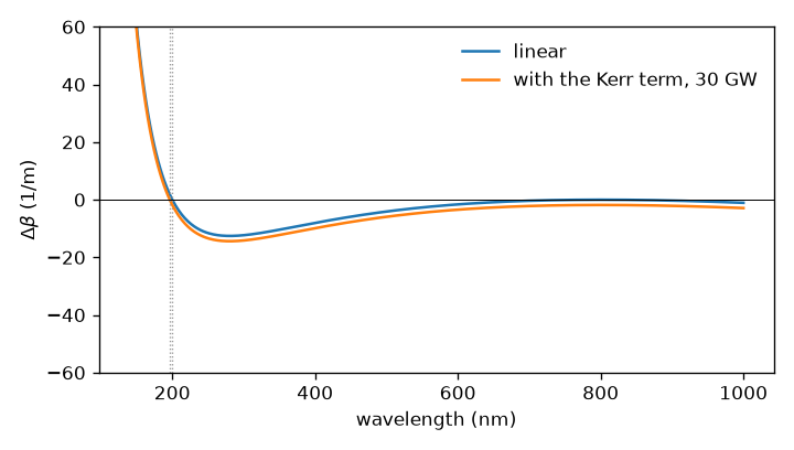
The phase mismatch of the fundamental mode of a 125 µm capillary filled with 1 bar of helium, for an 800 nm soliton, with and without the nonlinear wavenumber of a 30 GW soliton. The dispersive wave is phase matched where a curve crosses zero; the linear curve has a double zero at the pump because its carrier and group-delay terms have been subtracted. The nonlinear curve is shifted and need not vanish there.#
Two details of the search. The mismatch is sampled on 2048 frequencies across the
window and every sign change is refined with Brent’s method, so
lambda_rdw_all() returns every root in the window in order — a
mode with two zero-dispersion points has a dispersive wave on each side of the pump, and
a window that reaches to the red finds both — while lambda_rdw()
returns the longest of them, which on the default window is the short-wavelength wave
nearest the pump. And a window with no root raises
ToolsError, naming the window and the sign of the mismatch
at its ends, rather than returning a placeholder that would propagate silently.
Intermodal matching is one keyword: soliton_mode= gives the mode the soliton
travels in, and the first argument the mode the wave is emitted into.
Range warnings. The search evaluates the index across a window far wider than its
answer, and those probes are silent. The answer is not: a dispersive wave at 187 nm in a
silica capillary lies below the 210 nm of Malitson’s fit, and
MaterialRangeWarning says so, because the number then
rests on an extrapolated cladding index.
The pressure that tunes it#
pressure_rdw() inverts the calculation: the pressure at which
the dispersive wave is phase matched at a target wavelength, by Brent’s method between
\(10^{-6}\) bar and pressure_max. With peak_power the nonlinear coefficient follows the
pressure inside the search. pressure_zdw() does the same for the
zero-dispersion wavelength. The capillary is built once and re-evaluated at each density
through its parameterised form, rather than rebuilt with its equation of state at every
step, so a search costs milliseconds.
>>> from solprop.tools import lambda_rdw, pressure_rdw
>>> from solprop.modes import MarcatiliMode
>>> mode = MarcatiliMode(125e-6, "He", 1.0, cladding=1.45)
>>> f"{lambda_rdw(mode, 800e-9) * 1e9:.1f} nm"
'186.8 nm'
>>> f"{pressure_rdw(125e-6, 'He', 160e-9, 800e-9, cladding=1.45):.2f} bar"
'0.74 bar'
Both refuse a bracket without a root by name. pressure_rdw samples the pressure
range on 129 logarithmic and 129 linear points, then refines sign changes only
between admissible samples. With the constituent phase it recomputes \(\beta_2\),
\(\gamma\) and the scattering content at each pressure, excluding normal dispersion
and pressures below the first soliton threshold. Multiple roots are an error:
use pressure_limits=(lower, upper) within the overall (1e-6, pressure_max)
range to choose a branch. Sub-grid root pairs and narrow admissible intervals
can be missed; narrowing the bracket improves their resolution.
Designing a capillary for a soliton#
The usual question runs the other way round: given a core radius, a gas and a pulse,
what pressure and energy give a chosen zero-dispersion wavelength and a chosen soliton?
capillary_design() answers it in two steps. The pressure
places the zero (pressure_zdw()) and does not depend on the
energy. At that pressure \(\beta_2\) and \(\gamma\) are fixed, and
\(N^2=\gamma P_0\tau_0^2/|\beta_2|\) is linear in the peak power, so the energy follows in
closed form:
Exactly one target sets \(N\):
soliton_order, the conventional \(N\) itself. In normal dispersion it is still designed, as the conventional measure, and the result has no soliton content.soliton_count, a number \(M\) of solitons in the scattering content. The pulses with \(M\) solitons have areas \(S\in(M-\tfrac12, M+\tfrac12]\) (above); the design takes the middle, \(S=M\). That is the pure \(M\)-soliton, \(N=M\), for sech, and \(N=M\sqrt{\pi/2}\) for a Gaussian, as far as it can be from either threshold.largest_eigenvalue, the \(\eta\) of the largest constituent, which sets its width \(\tau_0/(2\eta)\) and its peak power \(P_0(2\eta/N)^2\). For sech \(N=\eta+\tfrac12\). For a Gaussian there is no closed form, so \(N\) is found by Brent’s method on the Gaussian eigenvalue. The bracket is \([\eta+\tfrac12,\ \eta+0.7]\): \(N-\eta\) falls from \(\sqrt{\pi/8}\approx0.627\) at the first threshold towards \(\tfrac12\) (0.579 at \(N=1\), 0.506 at \(N=10\)).
Holding \(N\) fixed holds the whole dimensionless content fixed. The count, the area and \(\eta\) depend on \(N\) and the shape alone, so changing the energy to keep \(N\) keeps the content too. The two targets on the content need anomalous dispersion at the pump and refuse a zero on its long-wavelength side. A Gaussian design and a sech design with the same FWHM and the same \(N\) have different energies, because each shape’s \(N\) uses its own natural width.
>>> from solprop.tools import capillary_design
>>> p = capillary_design(125e-6, "Ar", zdw_wavelength=500e-9, fwhm=10e-15,
...                      wavelength=800e-9, soliton_order=3.0, cladding=1.45)
>>> f"{p.pressure:.4f} bar, {p.energy * 1e6:.1f} uJ"
'0.0664 bar, 100.5 uJ'
>>> g = capillary_design(125e-6, "Ar", zdw_wavelength=500e-9, fwhm=10e-15,
...                      wavelength=800e-9, largest_eigenvalue=1.0, shape="gauss",
...                      cladding=1.45)
>>> f"N = {g.soliton_order:.4f}, eta = {g.soliton_content.largest_eigenvalue:.6f}"
'N = 1.5491, eta = 1.000000'
The result is the SolitonParams of
capillary_params() at the designed pressure and energy, with
the mode. pressure_zdw sets the limits: a single built-in gas, the HE_1m mode.
Antiresonant fibres from measured geometry#
The forward RDW solvers accept VincettiMode
as they accept any mode. Construct its lattice from the core radius, wall
thickness, inner resonator to core diameter ratio, and resonator count:
from solprop.modes import TubeLattice, VincettiMode
from solprop.physdata import n2
from solprop.tools import lambda_rdw_all, nonlinear_coefficient, pressure_rdw

radius = 20e-6
lattice = TubeLattice.from_inner_diameter_ratio(radius, 300e-9, 0.6, 6)
mode = VincettiMode(radius, "He", 2.0, lattice=lattice)
gamma = nonlinear_coefficient(mode, n2("He", pressure=2.0, wavelength=800e-9), 800e-9)
roots = lambda_rdw_all(
    mode,
    800e-9,
    peak_power=1e9,
    gamma=gamma,
    fwhm=30e-15,
    shape="gauss",
    wavelength_limits=(210e-9, 700e-9),
)
# For a selected root, invert with the same lattice and pulse:
if roots:
    pressure = pressure_rdw(
        radius,
        "He",
        roots[-1],
        800e-9,
        lattice=lattice,
        peak_power=1e9,
        fwhm=30e-15,
        shape="gauss",
        pressure_limits=(1.5, 2.5),
    )
Here \(D=2a\) is the inscribed core diameter and \(d\) is the inner resonator
diameter, so the model’s outer tube radius is \(a(d/D)+t\). Invalid dimensions
and overlapping resonators are refused. With lattice=None, pressure_rdw
keeps the capillary geometry. The Vincetti model’s fit limits, effective-area
approximation and material-range warnings apply
(the Vincetti model). An RDW root near a wall resonance
may suffer strong confinement loss: phase matching alone is not an efficiency
prediction. Inspect all roots and the mode’s loss, and narrow the wavelength
window when close resonances cannot be resolved by the 2048-point sampling.
Any guide, any parameter#
The pressure tools are written for the capillary. solve_parameter()
is their general form: it takes a builder, a function that returns the mode at a
trial value of any parameter (a radius, a pressure, a core size, a wall thickness), a
search range, and a target, and returns every value in the range that meets the target.
>>> from solprop.modes import MarcatiliMode
>>> from solprop.tools import ZDW, solve_parameter
>>> mode = MarcatiliMode(125e-6, "He", 1.0, cladding=1.45)
>>> roots = solve_parameter(
...     lambda radius: mode.at_parameters({"core_radius": radius}),
...     (20e-6, 500e-6),
...     ZDW(400e-9),
... )
>>> [f"{radius * 1e6:.2f} um" for radius in roots]
['89.49 um']
radius_zdw() is this search for the capillary, the radius
counterpart of pressure_zdw, with the same keywords and materials=:
radius_zdw("He", 1.0, 400e-9, cladding=1.45) is the same 89.49 µm.
There are three targets, each a frozen dataclass whose residual the search brackets:
target |
residual on the trial mode |
the builder returns |
|---|---|---|
|
\(\beta_2\) at the wavelength |
the mode |
|
the phase mismatch at |
the mode, or |
|
the pulse’s soliton order less |
|
A mode need not know its fill’s Kerr response, so a target that needs the nonlinear
coefficient asks the builder for it beside the mode, from
nonlinear_coefficient(); a builder that returns one serves a
linear target too, which ignores it. The search evaluates each mode at the launch
position z (zero by default).
How it searches. The residual is sampled on 129 linear values of the parameter and,
where the range is positive, 129 logarithmic ones, as pressure_rdw samples pressure.
Every sign change between two samples where the residual is defined is refined with
Brent’s method, to a relative tolerance of \(2\times10^{-12}\). A refined change is kept
only where the residual has fallen below a thousandth of its value at the bracket’s
ends: at a zero Brent’s method ends on a residual many orders smaller, while across a
pole, where a lossless resonance moves past the target, it converges onto the pole and
the residual diverges. Two roots closer than one sample are not separated; narrow the
range to resolve them. A search costs up to 258 builds and a few more for the
refinements, so a builder that re-evaluates one mode, as above, costs milliseconds per
value, while one that constructs a new capillary costs about 20 ms, and an antiresonant
or tabulated guide more.
Every root. The result is a DesignRoots: the roots in
ascending order, the range, the target and the number of builds. A design can have
more than one answer. The soliton order of a fixed pulse diverges at the pressure that
puts the zero dispersion at the pump, and is the conventional measure on both sides of
it, so an order can be met twice:
>>> from solprop.physdata import n2
>>> from solprop.pulses import SechPulse
>>> from solprop.tools import SolitonOrder, nonlinear_coefficient
>>> def build(pressure):
...     mode = MarcatiliMode(125e-6, "Ar", pressure, cladding=1.45)
...     kerr = n2("Ar", pressure=pressure, wavelength=800e-9)
...     return mode, nonlinear_coefficient(mode, kerr, 800e-9)
>>> pulse = SechPulse(wavelength=800e-9, fwhm=10e-15, energy=20e-6)
>>> roots = solve_parameter(build, (0.01, 5.0), SolitonOrder(4.0, pulse))
>>> [f"{pressure:.4f} bar" for pressure in roots]
['0.2770 bar', '1.3815 bar']
The first root is in anomalous dispersion, the second in normal dispersion, where the
pulse has no soliton. roots.pick(root) chooses one: "lowest" (the default),
"highest", or an index, negative from the end; an index out of range is refused,
naming the roots. A wall resonance of an antiresonant fibre gives its zero-dispersion
points in pairs in the same way: as the wall thickness passes the resonance, the
dispersion at a fixed wavelength turns from anomalous to normal and back, with further
sign changes inside the resonance band, and the search returns each of them.
No root. A range without a root returns no roots and the attainable range of
the target’s quantity, on a coarser grid of 17 linear and 17 logarithmic values: the
zero-dispersion wavelength nearest the target, the phase-matched wavelength nearest the
target, or the soliton order. pick then refuses with it:
>>> roots = solve_parameter(
...     lambda radius: mode.at_parameters({"core_radius": radius}),
...     (20e-6, 60e-6),
...     ZDW(400e-9),
... )
>>> roots.pick()
Traceback (most recent call last):
...
solprop.exceptions.ToolsError: no value between 2e-05 and 6e-05 gives a zero-dispersion wavelength of 400 nm: across it the zero-dispersion wavelength nearest the target (m) spans 1.98111e-07 to 3.29809e-07
A mode with no zero dispersion in 100 nm to 3 µm, or no phase-matched wavelength in the window around the target, contributes nothing to that range; when no value does, the refusal says the quantity is undefined across the range.
The pulse for an order. The other soliton design holds the mode and asks for the
pulse. \(N^2=\gamma P_0\tau_0^2/|\beta_2|\) is linear in the peak power, so
soliton_peak_power() is closed form, and
pulse_energy() turns the peak power into an energy, as
capillary_design does at its designed pressure:
>>> import numpy as np
>>> from solprop.modes import base
>>> from solprop.tools import pulse_energy, soliton_peak_power
>>> mode, gamma = build(0.2)
>>> beta2 = float(base.beta2(mode, np.array([2 * np.pi * 299792458.0 / 800e-9]))[0])
>>> power = soliton_peak_power(3.0, 10e-15, gamma, beta2)
>>> f"{power / 1e9:.3f} GW, {pulse_energy(power, 10e-15) * 1e6:.2f} uJ"
'1.947 GW, 22.09 uJ'
Designs under a material selection#
A run (materials) takes its gas index,
density and Kerr coefficient, and a numbered capillary’s default wall, from optmat by
default; a design computed from other data would name a pressure the run does not
reproduce. Every design tool that computes a gas or wall index or a Kerr coefficient
from a name therefore takes the same materials= keyword, with the same default,
MaterialSelection() —
soliton_params(), capillary_params(),
capillary_design(),
gas_ratio(), pressure_zdw(),
pressure_rdw() and radius_zdw() — and
resolves exactly as the capillary driver
does: a name, a fraction mapping and "air" (nitrogen and oxygen) through the
selection, the Kerr coefficient at the tool’s pump wavelength (a selection naming
another carrier is refused, as a run refuses it), and cladding=None as optmat’s
recommended fused silica. A pressure search takes each density from the selected
species’ own equation of state. A supplied Mixture and a caller’s mode are taken as
they are; the mixture carries its pressure and temperature, so a pressure= or a
temperature= other than its own beside it is refused (ToolsError), as a run refuses
them.
from solprop.tools import pressure_zdw

pressure = pressure_zdw(125e-6, "Ar", 600e-9)
# prop_capillary(125e-6, length, "Ar", pressure, ...) then has its zero-dispersion
# wavelength at 600 nm, to the tool's own accuracy; so does a run and a design under
# one explicit selection, MaterialSelection(...), passed to both.
A search samples pressures up to pressure_max, where an
optmat fill’s dilute law departs from its finite-density one; those probes are silent,
and the answer warns if it lies there.
How far to trust the estimate#
These are estimates made at one pressure and one peak power, and a run is neither. A
reduced resonant-dispersive-wave run is the honest example: 275 µJ in 7.5 fs at
800 nm into a metre of 125 µm capillary whose helium falls from 1.2 bar to vacuum. At the
entrance pressure the phase matching says 206 nm, or 201 nm with the nonlinear
wavenumber of the input pulse (nonlinear_phase="supplied_power"). The run puts its dispersive wave at 147 nm. Nothing is
wrong with either number: the pulse compresses on its way down the gradient and sheds
the wave where the gas has thinned, and 147 nm is phase matched at 0.62 bar, the
pressure that fill reaches three quarters of the way along. For a gradient, evaluate
the tools at the pressure where you expect the fission, not at the entrance. The test
suite checks this comparison against the run.
The design solvers, solve_parameter and its targets, were proposed and carried out by
SEP 41.