Plotting: the standard figures#

Use propagation maps to locate spectral broadening, compression or beam motion, then inspect slices and statistics at the relevant positions. A logarithmic map reveals weak features, but its colour scale alone does not tell you their energy. Compare bands quantitatively with the processing tools.

The RDW lesson develops the usual spectral, temporal and modal plots; the filament lesson adds spatial intensity and fluence. This chapter describes the standard figures and their units. Plotting functions accept an output object and return Matplotlib figures without calling show; slice plots also accept an ax for a supplied panel.

Display units#

These are conventions of the figure. Everything solprop.processing returns is SI (conventions.md §1); the conversion happens in solprop.plotting.style, once.

quantity	unit
distance along the fibre	centimetres
time and pulse duration	femtoseconds
wavelength	nanometres
frequency	petahertz
angular frequency	radians per femtosecond
energy	microjoules
power	auto-scaled, kilowatts to petawatts
intensity	terawatts per square centimetre
spectral energy density on a map	decibels below the peak

A hollow planar run is per unit width in y, so its powers and energies carry a /m in their labels (per_width()).

The propagation maps#

prop_2d() is the figure most runs are looked at through: the spectral energy density in decibels beside the instantaneous power, both against distance. A multimode run gets one figure per mode and a last one for the modal sum; a single-mode run gets one figure. The spectral abscissa is frequency by default and may be "wavelength" or "omega"; the colour scale runs down to db_min (−60 dB). The decibel scale is shared, normalised by the peak of the modal sum, so the modes are comparable, the sum’s map peaks at 0 dB and no map goes above it.

The bandpass reaches the temporal panel only: a window drawn on the spectrum it is displayed beside would be circular.

The spectral window spec_range is in the SI units of the abscissa, as everywhere in solprop.processing: metres on "wavelength", hertz on "f" and rad/s on "omega", so a frequency map can start at zero, which no wavelength range can say. The same holds for spec_1d and spectrogram. Left out, it is a fixed wavelength range converted to the abscissa; wavelength_to_axis() makes that conversion for anyone who thinks in wavelength:

from solprop.plotting import prop_2d, wavelength_to_axis
from solprop.processing import example_output

output = example_output()
prop_2d(output, "f", spec_range=(0.0, 2e15))
prop_2d(output, "omega", spec_range=wavelength_to_axis("omega", (600e-9, 1100e-9)))

import matplotlib.pyplot as plt
from solprop.plotting import prop_2d
from solprop.processing import example_output

figure = prop_2d(example_output(), "wavelength", spec_range=(600e-9, 1100e-9),
                 time_range=(-100e-15, 100e-15))[0]
figure.set_size_inches(9.5, 3.4)
figure.tight_layout()

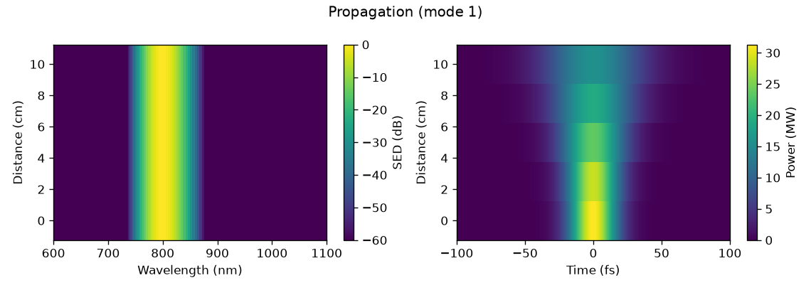
../../_images/plotting-prop-2d.png — The example run: a 30 fs Gaussian broadened by pure group-velocity dispersion. The spectrum does not move, which is what pure dispersion means, and the pulse doubles its duration.#

The slices#

time_1d() and spec_1d() draw one or more positions along the fibre: a colour per position, a dash pattern per mode (the patterns repeat when there are more modes than patterns), and the width at half maximum appended to each temporal legend entry. time_1d draws the power, the real field or its square; spec_1d draws the density on any of the three abscissae, logarithmic by default over six decades.

import matplotlib.pyplot as plt
from solprop.plotting import spec_1d, time_1d
from solprop.processing import example_output

output = example_output()
figure, (left, right) = plt.subplots(1, 2, figsize=(9.5, 3.4))
time_1d(output, [0.0, 0.1], time_range=(-120e-15, 120e-15), ax=left)
spec_1d(output, [0.0, 0.1], spec_range=(600e-9, 1100e-9), ax=right)
figure.tight_layout()

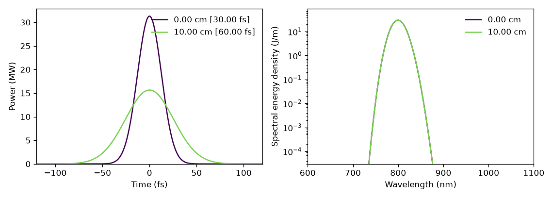
../../_images/plotting-slices.png — Time and spectral slices at the two ends of the example run. The spectrum is unchanged and the pulse is twice as long, as pure dispersion requires.#

time_1d() also takes transfer=, a linear optical element of solprop.optics, and transform_limit=, and draws the pulse after a compressor or at its limit (compression); spectrogram() takes transfer=.

plot_energy() follows the energy along the fibre in microjoules, with a linked right-hand axis in per cent of the total energy of every mode at the first plane, which is what a conversion efficiency means. Its limits are computed from the left axis’s, so the two axes always agree.

The statistics panels#

plot_stats() draws every statistic a run recorded, in two figures: what the pulse did, and what the waveguide and the gas were doing while it did it. Only the groups that have something in them are made, and a run with no statistics at all gives an empty list and no error.

A panel gets a logarithmic ordinate when its values are everywhere positive and span more than a decade. Per-mode statistics are drawn as one line per mode, named from the run’s own metadata.

from solprop.plotting import plot_stats
from solprop.processing import example_output

figure = plot_stats(example_output())[0]
figure.set_size_inches(8.0, 6.0)
figure.tight_layout()

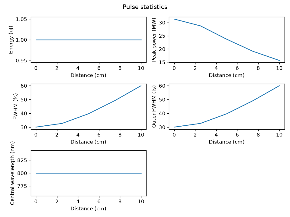
../../_images/plotting-stats.png — The pulse statistics of the example run. The energy is conserved, the peak power halves and the duration doubles, which is the whole of what pure dispersion does.#

Spectrograms#

spectrogram() gates the real field with a Gaussian and transforms at evenly spaced positions, through scipy.signal.ShortTimeFFT. The trade is the usual one: a gate of duration \(\tau\) resolves frequencies no better than \(1/\tau\), so a short gate shows when and a long gate shows what. The gate below is at the geometric mean of the transform-limited duration and the chirped one, which is where a linear chirp is most legible. By default the gate is a twentieth of the time range wide (gate_fwhm) and is placed at 256 positions across it (positions); log=True draws decibels below the peak. A spectrogram is of one field, so a multimode run must name the mode it means, and is refused if it does not. The map itself, without the figure, is get_spectrogram(): the gate positions, the spectral axis and the values, per unit of that axis, with the same gate and a bandpass= window.

import numpy as np
from solprop.grid import EnvelopeGrid
from solprop.output import MemoryOutput
from solprop.output.schema import GridRecord, RunMetadata, SavedPlane, StepperRecord
from solprop.plotting import spectrogram
from solprop.pulses import GaussianPulse

grid = EnvelopeGrid.from_limits(1.0, 800e-9, (400e-9, 2e-6), 4e-12)
tau0 = 30e-15 / (2 * np.sqrt(np.log(2)))
pulse = GaussianPulse(wavelength=800e-9, fwhm=30e-15, energy=1e-6).build(grid)
chirped = pulse * np.exp(-0.5j * 45 * tau0**2 * (grid.omega - grid.omega0) ** 2)

output = MemoryOutput()
output.open(
    RunMetadata(
        grid=GridRecord.from_grid(grid),
        modes=(),
        simulation_kind="mode_averaged",
        configuration={},
        stepper=StepperRecord(tableau="DOPRI5", controller={}),
    )
)
output.save(SavedPlane(z=0.0, field=chirped))

figure = spectrogram(
    output,
    time_range=(-1.2e-12, 1.2e-12),
    gate_fwhm=200e-15,
    spec_range=(700e-9, 950e-9),
)
figure.set_size_inches(6.4, 3.6)
figure.tight_layout()

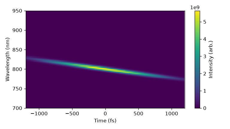
../../_images/plotting-spectrogram.png — A 30 fs pulse carrying 45 times its own duration of group-delay dispersion. Long wavelengths arrive first and short ones last, which is what normal dispersion does and what the optics sign convention says it should look like.#

The style helpers#

helper	what it does
`cmap_white()`	A colour map whose lowest colour is white, so that an empty map looks empty.
`cmap_colours()`	Evenly spaced colours for a family of lines.
`subplot_grid()`	A near-square grid of exactly the axes asked for; surplus ones are removed.
`power_unit()`	The factor and the label that put a power between one and a thousand.
`spectral_display()`	The factor and the axis label of a spectral abscissa.
`wavelength_to_axis()`	A wavelength range as SI limits on any of the three abscissae.
`corner_text()`	A panel label in a corner, in axis coordinates.
`fwhm_arrows()`	Two arrows and a label marking a trace’s width at half maximum.
`mode_labels()`	`HE11`, and the polarisation when the set mixes angles, from the mode records.
`per_width()`	The `/m` suffix a power or energy label takes on a run that is per unit width.

Mode names come from the structured metadata: a mode records the class it is and the arguments it was built from, so the label is read rather than parsed out of a printed description, and a change to how a mode prints cannot break it.

Cross-section drawings#

solprop.plotting.geometry draws the cross-section of a guide or a free-space grid: its outline, not its fields. A capillary is its gas-filled bore in a wall; an antiresonant fibre its tubes, to scale, inside a jacket; a step-index fibre or a graded-index provider its core in a cladding; a rectangular or planar guide its bore between walls or plates; and a radial, Cartesian, line or planar grid its medium with the absorbing collar its collar_fraction adds outside it. The cross-section figures of the spatial decompositions draw their outlines from it, so the manual and the library show one geometry.

None of the hollow-guide models carries a wall thickness: the wall enters only through the effective index. It is drawn WALL_FRACTION of the guide’s size thick, and so is an antiresonant fibre’s jacket. A direction the geometry leaves unbounded, a fibre’s cladding or the y of a planar guide or a line grid, is drawn to the extent you give, in metres. Everything else is to scale, at the position z along a guide whose radius or width varies.

import matplotlib.pyplot as plt

from solprop.modes import TubeLattice, VincettiMode
from solprop.plotting.geometry import draw

lattice = TubeLattice(wall_thickness=180e-9, tube_radius=9e-6, n_tubes=6)
fibre = VincettiMode(15e-6, cladding=1.45, lattice=lattice)
figure, ax = plt.subplots(figsize=(4, 4))
draw(ax, fibre)  # axes in micrometres, equal aspect
plt.close(figure)

name	what it does
`outline()`	The cross-section as shapes in metres, back to front: each a `Disc`, `Ring` or `Box` naming the region it fills.
`draw()`	Those shapes in a Matplotlib axes, in micrometres.
`thumbnail()`	A small square figure of a route’s representative guide or grid, with no axes, for a front end’s route picker; the pairs it draws are listed in `THUMBNAILS`.
`Palette`	The colours: a fill and an edge per region, a background and the dashed boundary, each a `#rrggbb` string; `LIGHT` (the default) and `DARK` are built in.

The colours are explicit rather than styled by a stylesheet, so a drawing looks the same in Matplotlib, saved as SVG, and in a Qt application. A thumbnail is a bare matplotlib.figure.Figure, made without pyplot: it needs no closing, saves to PNG or SVG with savefig at size pixels square, and shows in Qt through matplotlib.backends.backend_qtagg.FigureCanvasQTAgg.

import io

from solprop.plotting.geometry import DARK, thumbnail

icon = thumbnail("capillary", "mode_averaged", 96, palette=DARK)
buffer = io.BytesIO()
icon.savefig(buffer, format="png")  # 96 x 96 pixels, for a picker's icon

The geometry outlines were proposed and carried out by SEP 41.