Absorbing boundaries#

Both axes of the grid are finite and periodic, because both are sampled for FFTs. Energy that reaches the edge of the frequency window or the edge of the time window therefore does not leave the simulation: it wraps around and aliases onto the rest of the field. Absorbing boundaries attenuate light near the edges to reduce these artefacts. Their finite strength and width must be checked for the actual calculation.

They matter whenever the physics genuinely reaches the edge of a window — soliton self-compression, modulation instability, a dispersive wave walking out of the time window at a hundred femtoseconds per metre. The rest of the time they should do nothing at all, and saying so is part of their job.

This page covers solprop.boundaries: why the absorber is a rate rather than a mask, how its spectral and temporal parts are applied, what it costs, and how to tell when it is too weak. It is for anyone whose pulse, or whose spectrum, reaches the edge of its window, and for anyone who wants to know what the collars do to a run that never gets there. The collars it works from are built by solprop.grid and described in grids and Fourier conventions; why the absorber is a rate, and where its temporal part is applied, are also recorded among the design decisions. Which runs carry an absorber, and how to change it, is near the end. Where solprop’s absorbing boundaries differ from Luna.jl’s, the differences are listed in Noteworthy differences from Luna.

Rates, not masks#

The simplest absorbing boundary multiplies the solution by a fixed collar profile W after every accepted step. The cumulative absorption is then Wⁿ, where n is however many steps the adaptive controller happened to take — a number derived from rtol. Two things follow, and both are wrong:

the answer depends on the tolerance. Tightening rtol does not approach a limit, it increases the absorption. Refining sixteen-fold erodes the spectral wings fifty-fold.
the taper is not a taper. At realistic step counts Wⁿ is a brick wall at the edge of the flat region, and that brick wall is the limit the scheme approaches. It erodes genuine spectral wings.

An absorbing boundary must instead be an absorption coefficient per unit propagation distance, so that traversing a distance L attenuates by a factor that depends only on L and not on how the solver chose to subdivide it. solprop converts each collar profile into one. The spectral collar becomes

\[ \alpha(\omega) = -\frac{2 \log W(\omega)}{\ell}, \]

the rate that reproduces one multiplication by the window over the reference length ℓ; the temporal collar becomes the bounded profile

\[ \alpha(t) = \frac{A\,(1 - W(t))}{\ell}, \qquad A = 12.6, \]

the complement of its window (solprop.boundaries.TEMPORAL_ALPHA_LENGTH). Why the two differ is below.

The factor of two, and where it goes#

α is a power absorption coefficient, as everywhere else in solprop: power falls as exp(−αz), the field as exp(−αz/2), and the linear operator carries −α/2 (the conventions §2). The factor of two in the spectral definition is exactly what makes

\[ \mathrm{e}^{-\alpha \ell / 2} = W, \]

so that propagating through one reference length ℓ applies the collar profile to the field precisely once. The reference length is ℓ = length / boundary_N by default: “apply the window boundary_N times over the whole propagation”, with boundary_N = 20. The strength of the absorber is then a physical distance rather than a step count.

A slice of a run. That distance follows the grid’s length, so boundary_N gives a slice its own strength: a quarter of a run, rebuilt from its own grid, has a collar four times as strong as its parent’s, and the in-stage collar’s stability limit and the steps follow. boundary_length=parent.reference_length keeps the parent’s. A continuation through with_input is not affected, since it keeps the tables.

from solprop.boundaries import absorber
from solprop.grid import FieldGrid


def grid_of(length):
    return FieldGrid.from_limits(length, 800e-9, (400e-9, 2e-6), 400e-15)


whole = absorber(grid_of(1.0))
piece = absorber(grid_of(0.25))
kept = absorber(grid_of(0.25), boundary_length=whole.reference_length)
assert abs(piece.temporal_rate.max() / whole.temporal_rate.max() - 4.0) < 1e-9
assert kept.temporal_rate.max() == whole.temporal_rate.max()

Where each part goes is decided by what can be applied exactly:

part	mechanism	why
`α(ω)`	folded into the linear operator as `−α/2` before the cumulative operator is integrated	diagonal in ω, so the propagator applies it exactly over any sub-interval, at no cost
`α(t)`	the term `−α(t)E(t)/2` added inside every stage evaluation, masked to the active band	diagonal in t, so it cannot ride the propagator, and it belongs in the derivative so that the scheme integrates it at its own order
hard band limit	a 0/1 mask outside the active band	idempotent, and part of the definition of the band rather than an absorber

The hard limit sits outside the active mask ω_min/2 < ω < 1.1 ω_max, following the conventions §3. Putting it at the in-band mask instead would erase the collar the graded absorber acts on.

The two temporal schemes#

The temporal rate cannot be folded into the cumulative operator, and it cannot share the nonlinear polarisation’s transform either, because the UPPE prefactor is applied after that transform and the absorber is a rate on the field, not a polarisation. Two schemes represent it as a rate:

solprop.boundaries.nonlinear_absorber_term() — add −α(t)E(t)/2 inside every stage, with its own modal transform, masked to the active band. This is the default on the modal routes (capillary, waveguide and GNLSE).
solprop.boundaries.apply_split_step() — multiply the modal time-domain field by exp(−α(t)h/2) once per accepted step, followed by the hard band limit, because the product in time spreads content into every bin (on a field grid, chiefly the DC). One batched transform pair per step; the factors telescope, so the total is a rate whatever the step layout. Selectable as absorber_scheme="split_step", and the default on the spatial routes (radial, free-space and planar) unless their planes are interpolated (below).

Why the term and not the factor. The split factor is exact for the absorber alone, but applying it once per step is a Lie splitting of a term that does not commute with the linear flow — and a Lie splitting is first order. Measured on an N = 3 soliton launched into its collar, at 100, 200 and 400 fixed steps against the same problem at 1600, with the bounded temporal profile solprop uses:

scheme	relative error	observed orders
`split_step`	1.7e-3 · 8.6e-4 · 4.3e-4	1.00 · 1.00
`nonlinear`	3.5e-9 · 2.2e-10 · 7.1e-12	4.02 · 4.95

So the split factor caps a fifth-order scheme at first order wherever the collar removes anything, and makes the absorbed energy a function of rtol — the very defect the rate form exists to avoid, one level up. The conclusion does not depend on the temporal profile. With the capped logarithm as the temporal rate (below) the same ladder reads 7.657e-4 · 3.845e-4 · 1.912e-4 (orders 0.99 · 1.01) against 2.939e-5 · 1.278e-6 · 1.789e-8 (4.52 · 6.16), and quadrupling the steps moves the energy the split factor removes by 6.5e-5 of itself and the in-stage term’s by 9.0e-10. The in-stage term’s errors are four orders smaller under the bounded profile because the term it integrates is not stiff there.

What the term costs. One extra modal transform per stage, and one thing that needs watching: it is conditionally stable. The collar’s largest rate becomes an eigenvalue of the linearised problem, so an explicit method needs h·α/2 inside its stability region — 3.3 for DOPRI5. solprop.boundaries.stable_step() returns the limit, and translation refuses a problem whose replayed schedule or step floor is already past it, with a TranslationError naming the limit, the step and the remedies, rather than letting it diverge. A replay cannot reject a step: one that diverges for another reason stops with a ConvergenceError at the first step whose error norm is not finite, naming the step and the position, rather than writing NaN planes.

from solprop.boundaries import absorber, stable_step

boundary = absorber(grid)                 # ell = length / 20 by default
stable_step(boundary.temporal_rate)       # the longest step that will not blow up

An adaptive run finds the limit for itself — the rate reaches its ceiling only at the very edge of the window, where the field is negligible — so it costs steps and not correctness, and with the bounded profile only on runs shorter than about 2 · boundary_N steps. With the capped logarithm as the temporal rate it would cost steps everywhere: a ceiling of 60/ℓ on the collar’s last samples reaches the error estimate long before the stability limit, and on a reduced four-mode resonant-dispersive-wave capillary case costs 40 % more steps than the split factor, where the bounded profile takes the split factor’s count, 456 against 459. The split factor’s unconditional stability is the one thing it is better at, and why it stays selectable.

The two agree to first order in the step and differ at second, by (αh/2)²/2 — which is what the tests assert, and what would be false if the factor of one half were dropped.

The split’s crossing limit. The split damps the collar once per accepted step, at the step’s end. A step whose group-delay walk-off exceeds the collar’s width carries light through the collar and round the periodic window into the interior, where the factor does not touch it; on a nearly linear stretch the error estimate sees nothing, and a low-source run’s steps grow long. So under absorber_scheme="split_step" no step walks the light more than half the collar:

\[ h \le c\,\frac{w}{\max |\mathrm{d}\tau/\mathrm{d}z|}, \qquad c = 0.5, \]

with w the collar’s width and dτ/dz = ∂(β − β_frame)/∂ω the group-delay walk-off against the frame (solprop.boundaries.split_crossing_step(), solprop.boundaries.SPLIT_CROSSING), taken over the bins that hold light. Every (mode, frequency) bin’s walk-off is read from the translated operator into one of 128 rate buckets (solprop.boundaries.SplitCrossing, solprop.translate.linop.walk_off_buckets(): centred differences, one-sided at the active band’s edges and the last propagating bin before evanescence, a z-varying guide read at its operator’s own nodes, a coupled taper’s modes each at their own propagation constant from the flow’s generator); the fastest buckets that between them hold at most 1e-6 of the energy (solprop.boundaries.SPLIT_OCCUPIED_SHARE) are set aside, since all of that light wrapping would be a field error within the monitor’s default budget, and the fastest bucket left gives the rate.

At translation the rate is read from the launch. It holds an adaptive run’s dz_max, which is logged at INFO when it is lowered, and a fixed schedule whose longest step exceeds it is refused with a TranslationError that names the limit.
The boundary monitor reads it again from the state at every check, where each backend sums the state’s energy per bucket beside its other numbers, and the steps until the next check are capped by it, on every march, the native one included. Light that spreads into faster bins, a filament’s or a pulse’s broadening spectrum, so shortens the steps as it goes: on the 256-node radial filament of the benchmark suite the cap falls from 0.28 m at the launch to about 6 mm within 2 mm, above every step the run takes. A fixed schedule cannot shorten its steps, so a check whose cap falls below any of the schedule’s steps before the next check stops the run with a BoundaryError naming the cap, and a resumed schedule is held to the state it resumes from at once.
A run with boundary_check=None is held to the launch’s limit alone.

Read over every bin, outer transverse columns near their cutoff would set the limit even where they hold nothing: a 100 µm beam on a 1 mm radial grid of 512 nodes with a 70 fs collar took 109 steps over 5 cm instead of 25. Read where the light is, it takes 25 again, and the benchmark suite’s cases take the steps they took before. On a linear GNLSE pulse walking one window per metre, the limit takes Multistep from 14 steps of up to 0.3 m, which left 0.12 of the launch wrapped into the window, to 27 steps of 0.054 m, which leave 2e-4, the share a 1423 fs window should still hold. The in-stage scheme absorbs inside every stage and has no such limit.

Geometry, and the collar that is not one#

The collar geometry comes from the grid: the spectral collar rises over [ω_min/2, ω_min] and falls over [ω_max, 1.1 ω_max]; the temporal collar is symmetric about zero and lies outside the requested window. The grid widens the realised window to at least trange / (1 − 2f), with collar_fraction f = 0.1 by default, so the whole request is flat and the collar takes a tenth of the realised window beyond it at each end (grids). A collar inside the request would cut into light the run is meant to keep; the SEP 21 campaign measured that on a full-length Raman-soliton run, where it cost two orders of magnitude in accuracy.

Two settings change the geometry. collar_fraction=0 leaves no room for a temporal collar and realises the request alone, for a grid built by hand for a run without one; absorber=False keeps the room (below). collar_placement="inside" rebuilds the geometry solprop used before SEP 21: the window is the request rounded up, and the collar takes at least collar_fraction of it, inside the request when the rounding leaves too little slack. It exists to reproduce frozen comparisons and stored witnesses bin for bin.

A collar made only of the slack between the requested and the realised window would vanish whenever the transform size made the realised window equal to the requested one; the minimum fraction is what prevents that. solprop.boundaries.absorber() refuses a collar whose edge spans fewer than four grid samples: below that the discrete profile steps rather than tapers, the rate jumps to its cap in one sample, and the boundary is the brick wall the rate form exists to avoid.

The spectral cap, α·ℓ ≤ 60, has two jobs. The collar reaches exactly zero at the band edge and −2 log 0 is an infinity, which would put a NaN into the operator; and in the interaction picture the right-hand side is back-propagated by exp(+αΔz/2), which must stay finite. At 60 the field is attenuated by exp(−30), about 10⁻¹³, over one reference length — far below anything a propagation can represent. The temporal profile needs no cap: it is bounded by construction at 12.6/ℓ, and every rate is still validated against the ceiling of 60.

Why the temporal rate is not the logarithm#

The obvious temporal rate is the same capped logarithm as the spectral one. That is the right rate for a window that rides the linear operator for free, and the wrong one for a term in every stage: the Planck window falls so steeply that −2 log W is above 12 over the outer 14 % of each edge, which carries 73 % of the edge’s integrated attenuation, and the cap of 60 that keeps −2 log 0 finite becomes the largest eigenvalue of the linearised problem — the stability limit of the in-stage term and, through the error estimate, its step count. Lowering the cap alone halves the attenuation, because so much of it sits under the cap.

The profile A(1 − W)/ℓ keeps the integral — A = 12.6 reproduces the capped logarithm’s 6.3 per collar width per reference length to a few per cent — with a largest rate a fifth of the logarithm’s, every derivative continuous, and the attenuation spread over the edge instead of piled at its end. Measured on the reduced resonant-dispersive-wave case above: 456 steps against 637, and the in-window field differs between the two profiles by 3e-3 in the fundamental and 2e-3 in the second mode, on a case that carries 6 % of its fundamental in the collar. A case that holds a twentieth of its input field in the collar — a reduced hydrogen-filled capillary supercontinuum case — changes in kind between the two profiles: when a run’s physics happens inside the absorber, the result depends on the absorber, and the time window has to be widened.

Walk-off#

An absorber doing its job is silent, so solprop.boundaries.warn_walkoff() says when it stops being strong enough. A packet whose group delay drifts by Δτ over the whole propagation crosses the temporal collar at Δτ/L seconds per metre, so it spends dt/(Δτ/L) metres at each sample and accumulates

\[ \frac{L}{\Delta\tau}\,\frac{1}{2}\int \alpha(t)\,\mathrm{d}t \]

nepers of field attenuation on the way through. Below log(10³) — the field down by a thousand, the power by sixty decibels — the packet reaches the edge of the window still alive, wraps around, and appears at the front of the time window as an alias.

The group-delay span is the caller’s, deliberately. A prediction from the group delay across the whole simulation band, which on a grid running to four microns is dominated by band edges carrying nothing but shot noise, fires on almost every run — and a warning that is usually wrong is one people learn to ignore. A caller who passes the span of the band it cares about does not have that problem.

Sizing the collar from a walk-off#

A run that knows its drift can ask for the collar that stops it, rather than turn the drift into a strength by hand. Setting the attenuation above to Γ and the rate to α(t) = A(1 − W(t))/ℓ_c gives

\[ \ell_c = \frac{L}{\Delta\tau\,\Gamma}\,\frac{A}{2}\int (1 - W)\,\mathrm{d}t = \frac{6.3\,w\,L}{\Gamma\,\Delta\tau}, \]

since by the Planck taper’s symmetry W(x) + W(w − x) = 1 each edge of width w contributes w/2 to the integral. Both edges count: on the periodic axis they meet at the end of the window, and a packet re-enters the flat region only after crossing both. With Γ = log(10³), the condition warn_walkoff() checks, the default strength A·boundary_N = 252 stops a drift of 252 w/(2Γ) = 18.2 w (SEP 21 §4.2).

drift = 1.5e-12  # s, over the grid's length
walking = absorber(grid_of(1.0), walkoff=drift)
assert (walking.spectral_rate == whole.spectral_rate).all()  # the spectral collar stays
print(f"{walking.in_stage_length:.4f} m against {whole.in_stage_length:.4f} m")

walkoff fills collar_length (below) and nothing else. So:

Which length. The drift is measured over the grid’s own length. The rate depends only on the speed Δτ/L, so a slice given its own drift, a quarter of the length and a quarter of the walk-off, gets its parent’s temporal collar. Given its parent’s whole drift it gets a collar four times as strong.
Beside boundary_N or boundary_length. Neither conflicts with it, and neither is refused: they keep setting reference_length and the spectral rate, and walkoff sets the temporal rates. A slice that keeps both of its parent’s strengths passes boundary_length=parent.reference_length and its own drift.
Beside temporal=False. Refused: there is no temporal collar to size.
The window. It does not bound the drift. The attenuation depends on the collar’s width and not the window’s, and a drift of several windows is absorbed on its first crossing. It costs steps instead: at this strength an explicit method’s step is held to r w/(Γ v), about 0.48 w/v for DOPRI5 (r = 3.3, the stable step), so a long drift through a narrow collar is better served by a wider window.

A linear packet walking through this collar at the stated drift leaves exp(−2Γ) of its power, a millionth, to within the one sample the sizing’s integral leaves out of the period. The sizing assumes a steady drift over the run, as warn_walkoff does. Walk-off that starts late, after fission or as a soliton decelerates, crosses faster than the mean and is absorbed less, so the monitor stays the measurement. The default strength stays what it is for that reason: weak light that walks far needs its margin (SEP 21, decision D3).

import numpy as np
import matplotlib.pyplot as plt

from solprop.boundaries import absorber, split_step_factor
from solprop.grid import FieldGrid

grid = FieldGrid.from_limits(1.5, 800e-9, (90e-9, 4e-6), 400e-15)

fig, (ax_rate, ax_steps) = plt.subplots(1, 2, figsize=(9.5, 3.6))

# Only the trailing collar, which runs from the edge of the 400 fs request at 200 fs
# to the edge of the realised window near 256 fs: on the whole axis the flat request
# would take most of the width.
twin = ax_rate.twinx()
ax_rate.plot(grid.t * 1e15, grid.t_window, color="0.5", lw=1.2)
ax_rate.set_ylabel("collar profile", color="0.5")
ax_rate.set_ylim(-0.02, 1.05)
for index, strength in enumerate((20, 60)):
    rate = absorber(grid, boundary_N=strength).temporal_rate
    twin.semilogy(
        grid.t * 1e15, rate, color=f"C{index}", label=f"boundary_N = {strength}"
    )
twin.set_ylabel("absorption rate (1/m)")
twin.set_ylim(1e-2, 1e4)
twin.legend(frameon=False, loc="center right", fontsize="small")
ax_rate.set_xlabel("time (fs)")
ax_rate.set_xlim(190, 260)

# A point part way down the taper, where the collar profile is 0.9. As a rate the
# surviving field is exp(-alpha L / 2) whatever the step layout; as a per-step
# multiply it is 0.9^n, which is a different answer for every step count.
boundary = absorber(grid)
profile = 0.9
alpha = -2.0 * np.log(profile) / boundary.reference_length
distance = 0.3
counts = np.array([1, 2, 5, 10, 20, 50, 100, 200, 500, 1000])
as_a_rate = [
    float(np.prod(split_step_factor(np.array([alpha]), distance / n) ** n))
    for n in counts
]
ax_steps.loglog(counts, as_a_rate, "o-", label="as a rate")
ax_steps.loglog(counts, profile**counts, "s--", label="per-step multiply")
ax_steps.set_ylim(1e-20, 3.0)
ax_steps.set_xlabel("steps taken over 0.3 m")
ax_steps.set_ylabel("surviving field amplitude")
ax_steps.legend(frameon=False)

fig.tight_layout()

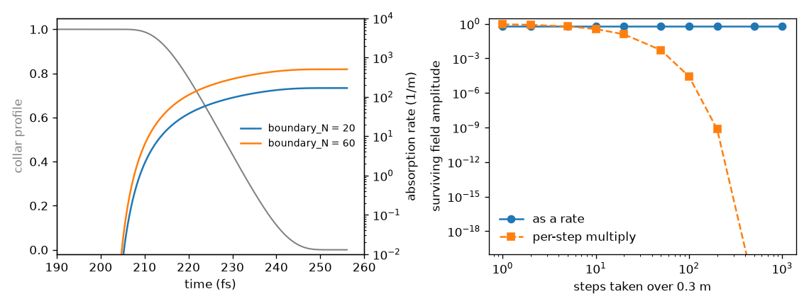
../../_images/boundaries-1.png — Left: the temporal collar of the RDW field grid and the absorption rate it becomes, for two absorber strengths. Right: the property the whole scheme exists for – the surviving field after 0.3 m is the same however that distance is subdivided, while a per-step multiply gives a different answer for every step count.#

Two lengths: the spectral rate and the in-stage collars#

A single length would set three things: the spectral collar’s strength, the ceiling 60/ℓ every rate is validated against, and the strength of the in-stage temporal collar, 12.6 (1 − W(t))/ℓ. (A free-space run’s real-space collar is designed separately, from a protected band and its width: transverse boundaries.) The two kinds of rate are applied very differently. The spectral rate is diagonal in ω and rides the linear operator, where it is exact and free whatever its strength; the in-stage collars are explicit terms, and their largest rate bounds the step an explicit method can take (the stable step). A measurement that needs a strong spectral absorber should not pay for it in steps.

So Absorber carries two lengths (SEP 22 §4.6):

reference_length, ℓ, sets the spectral rate and its ceiling 60/ℓ;
collar_length, ℓ_c, sets the in-stage temporal collar — its largest rate is 12.6/ℓ_c — and its ceiling 60/ℓ_c. None, the default, means reference_length, and a value equal to the reference length is stored as None. in_stage_length returns the length in force.

Take a 1 mm sample whose measurement calls for a spectral power rate of 10⁷ m⁻¹. The default ℓ = 50 µm caps rates at 1.2 × 10⁶ m⁻¹, so a single length would have to fall to 6 µm; the spatial collar’s peak would rise from 2.5 × 10⁵ to 2.1 × 10⁶ m⁻¹ and its DOPRI5 stable step fall from 26 µm to 3.1 µm. With two lengths the spectral rate moves and the collars do not.

collar_length is whatever sets the temporal collar’s strength: walkoff, when it is given, or else boundary_N or boundary_length. Nothing but the temporal collar reads it. A free-space run’s real-space collar, which SEP 21 and SEP 22 expected to share this length, is designed from its own protected band (SEP 40), so a walk-off moves no transverse strength.

A custom spectral absorber#

custom_absorber() adds a power rate of your own to a collar’s spectral rate:

from solprop.boundaries import absorber, custom_absorber

boundary = custom_absorber(grid, 1e7)                       # a scalar, 1/m
boundary = custom_absorber(grid, rates, collar=absorber(grid, boundary_N=60))
boundary = custom_absorber(grid, lambda omega: 1e6 * (omega > omega_cut))

The rate is a scalar, an array on the grid’s frequency axis or a callable of ω in rad/s; it must be finite and non-negative, and it is zeroed outside the collar’s band mask, where the operator is zero anyway. The collar is taken by value — None is absorber(grid), and any collar is accepted as it is, a spectral-only one included — and its temporal rates, band mask and in-stage strength are kept: the result’s collar_length is the collar’s own in_stage_length. Its reference_length stays the collar’s when the summed rate fits under the collar’s ceiling, and otherwise becomes 60 over the sum’s largest value, the longest length that admits it. The default collar already reaches its ceiling at the band edges, so any rate added there moves the reference length; the explicit collars never move. A zero rate returns the collar field for field, so its runs have the collar’s results and configuration hash.

The operator takes the sum, and Absorber.user_rate keeps the user’s share of it: spectral_rate stays the total, so the operator moves by no bit, and 0 <= user_rate <= spectral_rate holds on every bin. absorbed_power reports the share as its own custom channel and the collar alone as spectral, so what your loss took and what the numerical collar took read apart, and their sum is the power the spectral rate removes. A rate added twice adds its shares. A collar without one has user_rate=None, which the run record leaves out, so its record and hash stay; set, the share is recorded, since two splits of one total are not one run. absorber=False clears it with the rate it belongs to. In vacuum, on a linear beam, a bin’s energy falls by \(1-e^{-L\sum_i\alpha_i}\) and each rate’s share of that is \(\alpha_j/\sum_i\alpha_i\) (the statistic).

A spectral walk-off absorber#

A temporal collar cannot tell light that is merely late from light about to wrap, so it removes everything past the edge of its flat region. For a detector that integrates over time, that late light is signal. Where the walk-off can be predicted, a rate in ω can leave it alone and remove only the frequencies that would land on the part of the window that matters. This is a recipe, written with what the caller knows, and not a built-in.

The geometry. Light at ω walks from the frame by

\[ \Delta\tau(\omega) = \left|\beta_1(\omega) - \beta_1(\omega_{\rm frame})\right| L. \]

On a periodic window of length W, light that has walked but not wrapped is still exact physics. Let the pulse and any delay scan occupy the protected region |t| ≤ h. A packet launched at τ and walking later lands at τ + Δτ − W once it wraps, so it enters the protected region when Δτ ≥ W − h − τ; the worst launch, τ = +h, gives Δτ = W − 2h, and one walking earlier from τ = −h gives the same. So the rate has to be full by W − 2h: light just past it lands just inside the region, and a rate still rising there would let much of it through. It rises as a raised cosine over the h before that, and stays full beyond:

\[ \alpha(\omega) = \alpha_f\,P\!\left(\frac{\Delta\tau(\omega) - (W - 3h)}{h}\right), \qquad P(x) = \tfrac12\bigl(1 - \cos\pi\,\mathrm{clip}(x, 0, 1)\bigr). \]

Bins in the rise lose light that would not have reached the region. That is the price of the guarantee, and the check below measures it.

The strength. Power falls as exp(−αz), so light launched at the entrance leaves with exp(−α_f L). Light born part-way is the harder case. What walks Δτ over the whole length reaches the protected region after (W − 2h)/Δτ of it, when it has lost only that share of the exponent. To hold a power fraction f for all of it, take the largest walk-off the run carries, as warn_walkoff’s span is taken:

\[ \alpha_f = \frac{\ln(1/f)}{L}\,\frac{\max(\Delta\tau,\,W-2h)}{W - 2h}. \]

f = 10⁻⁶ is the collar’s own Γ = log(10³) in field. All of it sits in the linear operator, where it is exact and needs no transform pair, and it adds no in-stage stability limit.

import numpy as np

from solprop.boundaries import custom_absorber
from solprop.constants import C
from solprop.driver import Simulation, SimulationSettings
from solprop.grid import LineGrid
from solprop.physdata.glasses import fused_silica
from solprop.pulses import GaussianPulse, SpatialPulse
from solprop.spatial import SpatialMedium
from solprop.stats import StatsSpec
from solprop.stepper import PIController, RungeKutta

length = 40e-6
medium = SpatialMedium(fused_silica())
grid = FieldGrid.from_limits(length, 800e-9, (150e-9, 2e-6), 120e-15, collar_fraction=0)
window = grid.n_t * grid.dt
protected = 25e-15  # h: the pulse and the delay scan


def beta1(omega):
    """The group delay per metre of the medium, s/m."""
    index = np.real(medium.index(omega))
    return (index + omega * np.real(medium.dindex_domega(omega))) / C


active = grid.active_mask
delay = np.zeros(grid.n_omega)  # what walks furthest is what the run carries
delay[active] = (
    np.abs(beta1(grid.omega[active]) - beta1(np.array([grid.omega0]))) * length
)
carried = delay[grid.inband_mask].max()

arrival = window - 2 * protected  # the earliest walk-off to land on the region
onset = arrival - protected
full = np.log(1e6) / length * max(carried, arrival) / arrival
walkoff_rate = (
    full * 0.5 * (1 - np.cos(np.pi * np.clip((delay - onset) / protected, 0, 1)))
)
boundary = custom_absorber(grid, walkoff_rate, collar=absorber(grid, temporal=False))

For a guide, delay comes from solprop.modes.base.beta1() with the mode and the frame’s omega0. On a grid whose collar fraction is zero, as here, the window is the request, since a spectral-only collar needs no room in time. Nothing the run carries is absorbed when W ≥ 3h + max Δτ; leave some margin on top, for what the linear estimate misses. A window shorter than that trades light for samples, and the check below says how much. Here it is far shorter, so the rate starts at about 193 nm and is full from about 175 nm.

The limits.

It is a prediction from linear dispersion. It knows nothing of the nonlinear changes of group delay: the soliton self-frequency shift, the plasma blue-shift, cross-phase modulation. It suits weakly nonlinear runs, and a strongly nonlinear run keeps the collar and warn_walkoff, which need no dispersion model.
It assumes light travels the whole length. The rate acts on a frequency wherever it is, so light born part-way that would never wrap is absorbed as well. That errs on the side of safety for the protected region, and it is a loss of signal for the band.
It acts on a frequency and not on a time. A bin past the onset is lost at every delay, also where light launched at −h would still sit inside the protected region at the end. So the loss depends on the delay, and it is worst for the launch furthest from wrapping.
A narrower rise keeps more of the band, since a width s in place of h needs only W ≥ 2h + s + max Δτ, but it spreads the edge further, as the next point says.
It rests on the group-delay picture. A rise over s in delay is a rise over s/(|β₂|L) in frequency, whose edge spreads in time by about |β₂|L/s, so it needs s² ≫ |β₂|L where the rate rises.
It needs the caller’s protected half-width. The rate cannot find it from the run.
One (n_omega,) rate must cover every mode and every transverse column. A multimode or strongly angular run needs the worst case over them, which absorbs more of the rest.

How it costs less. With no temporal rate the run compiles no temporal pass, under either scheme (below). On a Kerr run over ten steps on native CPU, with the fields agreeing, that took about 10 % off the per-step time of the collar under the split scheme, the spatial routes’ default, and about half off the in-stage term, on the same grid (the ledger).

Check it per band. A fraction of total power hides what this rate does. Weak short-wavelength light can lose most of its band while the run’s energy moves by 10⁻⁵, and the band’s loss is what says the window is too short. The rate is diagonal in ω, so each bin loses α(ω) S(ω, z), with S the beam_spectrum, integrated in z. That statistic is taken at saved planes and not between them, so the integral runs over the planes, with an error of about (α Δz)²/12 of a bin’s loss by the trapezoid. Dividing by what the band kept and lost together counts light the run generated part-way as well as light it launched. absorbed_power has the user’s share as its custom channel, but over the whole beam: only this product reads it per band. A lossy medium’s own absorption is a further channel: fused silica absorbs at these wavelengths, and what it takes appears in neither count.

planes = np.linspace(length / 32, length, 32)
settings = SimulationSettings(
    controller=PIController(rtol=1e-6, atol=1e-14),
    save_planes=planes,
    dz_max=length / 32,
    dz_init=length / 32,
    integrator=RungeKutta(),
    backend="numpy_ref",
    absorber=boundary,
    boundary_check=None,
    stats=StatsSpec(names=("beam_spectrum",)),
)
beam = SpatialPulse(GaussianPulse(wavelength=170e-9, fwhm=20e-15, energy=1e-9), 1e-3)
space = LineGrid(4e-3, 16)
output = Simulation.from_free(
    grid, space, medium, [], beam, settings=settings, noise=None
).run(progress="none")

# (n_z, n_omega), J/(rad/s) per metre of y
spectrum = np.asarray(output["stats/beam_spectrum"])
z = np.asarray(output["z"])
lost = np.trapezoid(walkoff_rate * spectrum, z, axis=0)
collar_lost = np.trapezoid(
    (boundary.spectral_rate - walkoff_rate) * spectrum, z, axis=0
)
wavelength = 2 * np.pi * C / np.where(grid.omega > 0, grid.omega, np.inf)
band = (wavelength >= 150e-9) & (wavelength <= 190e-9)
share = lost[band].sum() / (
    lost[band].sum() + collar_lost[band].sum() + spectrum[-1, band].sum()
)
print(f"the walk-off rate took {share:.2f} of the 150-190 nm band")

A spectral-only collar#

absorber(grid, temporal=False) builds a collar with the spectral rate and the band mask of a full collar and no temporal part: its temporal rates are zero arrays on both time axes and its record says temporal: False. Any collar whose temporal rates are all zero, however it was built, crosses the seam as no temporal absorber (temporal_rates()), so the kernels compile no temporal pass under either scheme: no in-stage term, no split pass and its transverse transform pair, and the first-same-as-last stage recycled. absorber_scheme is still recorded and applies to nothing, and its refusal of interpolated planes does not fire. The grid is unchanged. Measured on a Cartesian envelope grid of 192 × 192 × 300 with a spectral-only collar, the pass that compiling away removes cost 1.2–1.6 times a step on native CPU (SEP 22 §3; the phase-1 re-measurement is in its implementation record). Under the in-stage scheme the zero rate only added zeros, so a run is unchanged; under the split it differs by the transform pair’s rounding.

A spectral-only collar is passed as absorber=absorber(grid, temporal=False); a keyword that turns both soft collars off on the fibre entry points is SEP 21’s.

The transverse boundary#

The collars above act on time and frequency. A free-space run’s transverse boundary is its own (SEP 40): a wall or a wrap at the grid’s outer size, a safety ramp in the transverse wavenumber on every geometry, which rides the linear operator exactly like the spectral rate, the monitor’s transverse edge, and, on request, a designed real-space collar, spatial_absorber=SpatialAbsorber(...) (SpatialAbsorber). It is independent of the Absorber and its lengths: transverse boundaries and grid sizing and the transverse safety ramp.

Which runs carry one, and how to change it#

entry point	absorber by default
`prop_capillary`, `prop_waveguide`, `prop_gnlse` and their `Simulation.from_*` builders	the grid’s default collar, `absorber(grid)`: spectral and temporal, `boundary_N = 20`, applied in every stage
`prop_radial`, `prop_free`, `prop_planar` and their builders, whose settings declare none	the same temporal and spectral collar, applied once per accepted step (`absorber_scheme="split_step"`) unless planes are interpolated; the transverse boundary is the safety ramp and the monitor’s edge, with a real-space collar only on request (`spatial_absorber`, SEP 40)
a `Simulation` built directly with its own `SimulationSettings`	none unless `SimulationSettings(absorber=...)` is given

Every prop_* entry point takes absorber= and absorber_scheme=. Pass absorber(grid, boundary_N=60) for a stronger collar, absorber(grid, boundary_length=...) to fix the reference length ℓ directly, and absorber=False for none: both soft collars, temporal and spectral, are switched off and the hard band mask is kept (solprop.boundaries.no_absorber()). The built grid keeps the collar’s room, so a run without an absorber shares the grid of the run with one, and the Raman response’s tail taper and the held plasma current’s gate, which read the collar’s width, keep their samples whatever the transform size rounds to. On the spatial interfaces absorber=False leaves the transverse collars as they are. absorber=None means “build the default”, not “no absorber”; a scheme beside absorber=False, or a keyword that contradicts what a spatial run’s settings already declare, is refused.

The spatial routes apply the temporal collar by the split scheme unless the settings name a scheme or interpolate their planes, which the split refuses: on the spatial cases of the performance-tracking suite the in-stage collar took 1.2 to 4.6 times the steps of the split one, at equal or worse accuracy inside the requested window (SEP 21). The split is unconditionally stable, so a fixed schedule on a spatial route keeps its collar, within the split’s crossing limit.

An absorber given explicitly does not switch on the real-space transverse collar, which is asked for on its own with spatial_absorber.

Watching the window’s edges#

The tutorial Is my time window big enough? sizes a window with what follows, on a short fibre whose Raman soliton walks towards the late edge.

Every run watches its time window (solprop.monitor.BoundaryCheck, on by default through SimulationSettings.boundary_check). At the launch and at every committed step it measures the share of the field’s energy in the outer 5 % of the realised window at each edge, the guards, and in the collar:

from the launch on, a guard occupancy whose square root exceeds the field-error budget (1e-3 by default, a millionth of the energy) warns once (BoundaryWarning), and ten times the budget (a ten thousandth) stops the run with BoundaryError; at the launch that means the window clips the input, which can seed spurious radiation, and the run is refused before its first step. Light the launch puts in the collar alone is absorbed, and the end of the run reports it;
at the end, the fraction of the launch energy the temporal collar removed is logged, and warns when its square root exceeds the budget. Weak spectral features can matter at far smaller fractions than that: the record is there to read.

How often, and what it saves. While some guard or the collar holds more than a tenth of the budget (as a field amplitude), every committed step is checked. While the edges are quiet, a step is checked every eighth step or after length / 256 of the guide, whichever comes first, and the state of every saved plane is checked regardless. The collar itself stays in every stage.

The quiet collar, on request. BoundaryCheck(quiet_collar=True) also leaves the in-stage temporal collar’s term, whose transform is a stage’s largest cost after the response’s, out of the stages while the collar is quiet: while it held less than 1e-12 of the field’s energy, the shot-noise floor included, at two checks in a row. A check that finds light in it puts the term back at once. While the term is out no step is longer than length / 256, so light cannot cross into the collar unabsorbed within one long step, and the exponential Adams march no longer limits its order by the collar’s stability; the first step after the term returns is held to that limit. Under input noise the floor alone fills the collar far above the threshold, so the option only acts on noise-free runs; on a 2 cm noise-free GNLSE Raman/shock run whose pulse stays clear it saved 6 to 9 % per step across native and the since-retired numba_cpu (Apple M5 Max). It is off by default because a run cannot know in advance whether its light stays clear, and an omission judged too early is an error nothing reports (ADR-057). It applies to binary64 modal and radial stages with the in-stage scheme; the split scheme, the low-storage march, the general modal route, coupled flows, a real-space collar, single precision, and the Cartesian, line and planar routes, whose stages keep the term regardless, always keep the collar. The record’s collar_left_out_checks counts the checks that found it out.

Above the shot-noise floor. Input noise, on by default, puts one photon per mode across the whole window, guards and collar included. Light below that floor cannot be told from the vacuum, so the monitor judges what lies above it: from each region’s energy it subtracts three times the floor’s expected share (the floor is uniform in time on average, and three times its expectation clears its fluctuation in a narrow guard), and from the collar’s removal the floor’s expected removal, up to the floor itself: the input noise puts one floor in at the launch and never adds to it, so the floor cannot lose more than that, however long the run. A weak launch is therefore not stopped for its own noise, while light well above the floor that reaches an edge still is. Light that arrives at an edge, or leaves through the collar, weaker than the vacuum’s own share of it is not reported.

What the monitor saw is kept in the run’s execution record, under boundary_monitor: the launch occupancies, the largest guard and collar occupancies and where the guards peaked, and the removed fraction, all above the floor; beside them the floor’s share of the launch energy (noise_floor) and the whole field’s largest guard share and removed fraction, floor included (raw_guard_max, raw_removed_fraction). Under planes it keeps one row per saved plane: z, the collar occupancy there, each guard’s largest occupancy since the previous plane, and the removed fraction so far. The record is rewritten at every saved plane without the rows, which the closing record (complete, failed or out of budget) carries, so a file does not grow with the square of its planes. Beside them are the thresholds the execution ran under (guard_fraction, budget, stop_factor, quiet_collar) and the launch’s energy in the monitor’s own units (launch_energy).

Under the in-stage scheme the removed fraction is integrated along z by the trapezoid. Under absorber_scheme="split_step" every backend adds up, in its own step finish, what each accepted step’s split takes of the power it finds, P(1 − e^{−αh}), so the removal is exact on every step, checked or not. Read back from the state the split leaves, the same removal would multiply whatever the band mask left deep in the collar by e^{αh}, into removals larger than the launch and false warnings.

The same finish keeps the energy and the guards’ and collar’s energies of that power taken halfway through the split’s factor, P e^{−αh/2}, and under the split every share of a check is judged on them, the no-light test included; a backend whose reading after a step lacks them is refused rather than judged on the state the split left. The state the split leaves has its guards, deep in the collar, damped by e^{−αh}, about e^{−10} at an adaptive step, so a pulse walking out showed nothing there and ran to the end of its fibre; the state before the split holds what walked into the guard during the step unabsorbed, and stopped the same pulse 40 % early. Half the factor is the symmetric (Strang) splitting’s state at the step’s end, second order in the step where the one-sided split is first. On a GNLSE pulse walking out of its window, the split’s stop falls within 1 % of the in-stage scheme’s at every dz_max from adaptive to 2.5e-4 m, and a radial one’s within 6 %.

A check reads five numbers of the state, its energy and the four weighted energies above, and each backend forms them where the state lives: on the GPU for mlx and a device build of native, in compiled code for native on the CPU, and with NumPy for numpy_ref, the reference the others are tested against. The field is not copied to the host to be watched.

A resumed run continues the record: the state it resumes from is checked by the first step, not judged as a launch, so a run stopped at an edge can be resumed under a relaxed check (the check is not part of the resume key; the quiet-collar opt-in is). The totals, the launch occupancies, the quiet collar’s state and the rows of a closing record are restored, so the removed fraction and the guard maxima continue against the original launch, and resumed_at lists where the run was resumed. A run killed without a closing record restores its totals, and its rows start again at the resume. The record continues from the latest execution that kept one: an execution killed before its monitor started, or run with boundary_check=None, is passed over, and the stretch it ran unwatched is listed under unwatched as [start, end] in metres, because what left the window there is unknown rather than zero. The record also keeps the signed removal (removed_signed) and the floor’s expected removal (floor_removed_fraction), so that a resume continues from the same numbers the whole run would hold.

On a free-space run the monitor also watches the transverse edge (SEP 40): the energy in the outer 5 % of the grid’s outer size above its launch value with no collar, and what returns with a requested one, at BoundaryCheck’s levels or its own transverse_budget, which relaxes the transverse edge without relaxing time. Its reads are spaced as a ceiling on the step, and its record joins the monitor’s under transverse, with a transverse_status that only reads clear for a run that read its edge at the required spacing and found nothing (transverse boundaries).

SimulationSettings(boundary_check=None), or boundary_check=None on any prop_* function or Simulation.from_* constructor, watches nothing; a BoundaryCheck with a larger budget or stop_factor relaxes it.

A worked example#

import numpy as np
from solprop.boundaries import absorber, apply_band_mask, apply_split_step, warn_walkoff
from solprop.grid import FieldGrid

grid = FieldGrid.from_limits(1.5, 800e-9, (90e-9, 4e-6), 400e-15)
boundary = absorber(grid, boundary_N=20)

# The spectral rate goes into the linear operator as -alpha/2. Here the temporal rate
# is applied to the time-domain field once per accepted step: the `split_step` scheme,
# which `absorber_scheme="split_step"` selects (the default applies it in every stage).
field = np.ones((1, 1, grid.n_t))
field = apply_split_step(field, boundary.temporal_rate, step=0.01)

# The hard band limit is a separate, idempotent multiply on the spectrum.
spectrum = apply_band_mask(np.ones((1, 1, grid.n_omega)), boundary.band_mask)

# And the run says so if the absorber is too weak for the walk-off it will produce.
warn_walkoff(grid, group_delay_span=1e-12)   # SolpropWarning: widen trange, or ...